Interaction Menu #

The Interaction menu contains the following options:

• Constraint
  • Create.
  • Edit.
  • Duplicate.
  • Swap Master/Slave.
  • Merge by Master/Slave.
  • Hide.
  • Show.
  • Delete.
• Contact
  • Surface Interaction:
    • Create.
    • Edit.
    • Duplicate.
    • Delete.
• Contact Pair:
  • Create.
  • Edit.
  • Duplicate.
  • Swap Master/Slave.
  • Merge by Master/Slave.
  • Hide.
  • Show.
  • Delete.
• Search Contact Pairs.

Available constraints include:

• Point spring:
  • Name.
  • Region.
  • Stiffness:
    • K1 – stiffness per node in the X direction.
    • K2 – stiffness per node in the Y direction.
    • K3 – stiffness per node in the Z direction.
  • Color.
• Surface spring:
  • Name.
  • Region. – Stiffness per area: No/Yes
  • Stiffness:
    • K1 – stiffness in the X direction.
    • K2 – stiffness in the Y direction.
    • K3 – stiffness in the Z direction.
• Color.
• Compression only:
  • Name.
  • Region.
  • Spring stiffness.
  • Tensile force.
  • Offset.
  • Nonlinear: No/Yes.
  • Color.
• Rigid body:
  • Name.
  • Reference point.
  • Region.
  • Color.
• Tie:
  • Name.
  • Position tolerance – the largest distance from the master surface for which the slave nodes will be included in the tie constraint (default: 2.5% of the typical element size).
  • Adjust – projection of the slave nodes on the master surface.
  • Master region.
  • Slave region.
  • Master surface color.
  • Slave surface color.

The compression-only constraint internally uses GAP elements connected to other finite elements via *EQUATION. The Offset parameter enables the offset of the ground node of GAP element away from the model for better visualization of the results. In the results, GAP elements are merged into one part. IMPORTANT: geometric non-linearity (NLGEOM) should be enabled when using the compression-only constraint. Otherwise, the compression-only support has 1/2 of the assigned stiffness and acts as a surface spring support. Setting the Nonlinear option to Yes also makes it possible to avoid this linearization by adding a dummy nonlinear material to the input file.

The rigid body constraint requires a reference point since it constrains the motion of the selected nodes to the motion of the reference point. It is used to define a selected region as infinitely rigid (non-deformable). For example, it’s often used when modeling manufacturing tools. However, it may also serve as a way to apply moments and remote loads to models. Rigid body constraint is the only way to apply a torque to the surface of a solid part (since solid element nodes don’t have the rotational degrees of freedom).

The tie constraint works like a bonded/welded contact. It connects two surfaces in such a way that they can’t separate or move relative to each other during the analysis, they are permanently connected. Tie constraint is often used to connect parts with dissimilar meshes.

Contact is a more complex form of interaction between two surfaces than the tie constraint. It allows the transfer of forces between touching surfaces. However, contact is a highly nonlinear phenomenon and requires careful usage as it may cause convergence issues. When defining contact, a surface interaction must be created first. Three options are available:

• Surface behavior – behavior of the contact in the normal contact direction (pressure-overclosure relationship)
  • Hard.
  • Linear.
  • Exponential.
  • Tabular.
  • Tied.
• Friction – behavior in the tangential direction
  • Friction coefficient.
  • Stick slope.
• Gap conductance – thermal conductance across the contact interface
  • Constant
  • Tabular – pressure and temperature dependent When the surface interaction is created, the contact pairs can be defined. The options here are as follows:
• Name
• Surface interaction
• Method
  • Node to surface – uses node-to-face penalty formulation.
  • Surface to surface – uses face-to-face penalty formulation.
  • Mortar – uses formulation with Lagrange multipliers, typically more accurate but requires more time to solve and may cause convergence issues. – Linear mortar – should be used only when Mortar fails.
  • PG linear mortar – should be used only when Mortar fails.
• Small sliding – available when Node to surface method is selected
• Adjust – projection of the slave nodes on the master surface.
• Adjustment size – distance inside which the slave nodes are projected to the master surface.
• Master region \ Slave region
• Master surface color \ Slave surface color

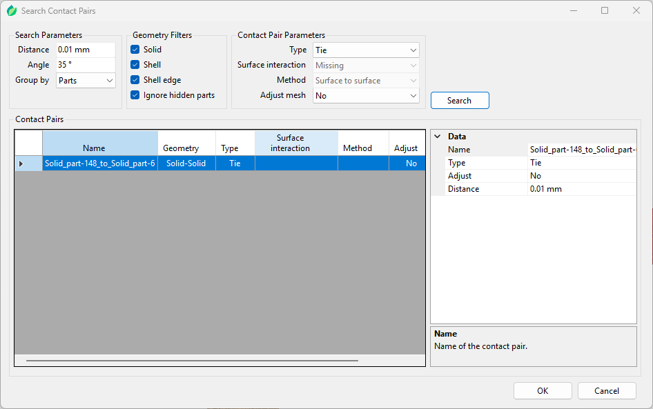
Figure 5: Search Contact Pairs tool

The Search Contact Pairs tool with exemplary input is shown in Figure 5. This tool allows users to automatically create contact pairs and tie constraints. Upon clicking the Search button the tool searches for surface pairs that meet the following criteria:

• distance between them is smaller or equal to the specified distance.
• angle between them is smaller or equal to the specified angle.

In addition to these criteria, user may choose whether the pairs are grouped by parts or not. Before performing the search, one can change the type of interaction (Contact or Tie), specify previously created contact property definition and choose the type of contact (surface to surface or node to surface). For both contact and tie creation, it’s possible to enable or disable adjustment. After the search, users can still change the aforementioned settings (as well as position tolerance and name of the pair) using the Data window on the right side of the tool. In addition, right clicking on the pair in Contact Pairs window brings an option to swap master and slave surfaces. When more than one pair is selected, an option to merge by master/slave also becomes available. Pairs can be removed from the list (and thus prevented from being created) by selecting them and pressing Delete .

Amplitude menu #

The Amplitude menu contains the following options

• Create.
• Edit.
• Duplicate.
• Delete.

The following amplitude types and settings are available:

• Tabular – can be used to specify the time/frequency – amplitude value data points
  • Properties
    • Name
    • Time span: Step time/Total time
    • Shift time
    • Shift amplitude
  • Data points – tabular data in form of time/frequency-amplitude pairs

Initial Condition Menu #

The Initial condition menu contains the following options:

• Create.
• Edit.
• Duplicate.
• Preview.
• Delete.

The following initial condition types and settings are available:

• Temperature – can be used to specify the temperature at the beginning of a thermal or thermomechanical analysis
• Name.
• Region.
• Temperature.
• Velocity – can be used to specify the velocity at the beginning of a dynamic analysis
  • Name.
  • Region.
  • Velocity components:
    • V1 – velocity in the X axis.
    • V2 – velocity in the Y axis.
    • V3 – velocity in the Z axis.
• Magnitude – resultant velocity (it’s calculated automatically when the components of the velocity are specified).